
An instantaneous snapshot of space makes it possible to identify zones of compression and decompression in the air. Physically, compression is the local accumulation (within a small volume) of air molecules: pressure increases. Conversely, decompression corresponds to the molecules moving apart from one another. These are therefore elastic collisions between molecules. These collisions (at the microscopic scale), and therefore the acoustic disturbance (at the macroscopic scale), propagate from point to point at a certain speed called the speed of sound (c) (in metres per second (m/s)).
At a given instant t, and given the duration T of one cycle, the latter will extend spatially over a certain distance, materializing what is called the wavelength λ of this variation (following figure). Thus, the relation is: $$lambda = c.T = c / F$$
(c), the propagation speed, is constant. Therefore, the higher the frequency (high-pitched sound), the smaller the wavelength: a few centimetres. The lower the frequency (low-pitched sound), the greater the wavelength: a few metres.
Acoustic waves, which are complex combinations of frequencies F and therefore of wavelengths λ ranging from a few centimetres to a few metres, will be sensitive to the dimensions of the obstacles they may encounter during propagation. These spatial properties also characterize the radiation of the sound sources that produce these waves.
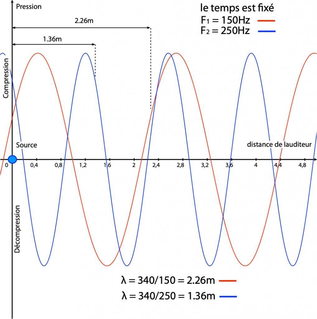
The illustration above highlights the spatial dimensions of one cycle of periodic variation. They can range from a few metres to a few centimetres depending on frequency. Note that at the source location ((d=0)), the contributions (F_{1}) and (F_{2}) are non-zero and do not have the same value. This difference in value — called the difference at the origin (at the source) — is referred to as the phase difference. In other words, this is the phase (denoted (phi) or (varphi)), or more precisely the initial phase (at the origin of time and space).
Returning to a local approach (as a function of time only), the equation for a sinusoidal variation seen earlier can be rewritten and generalized for a contribution (i):
(p_{i}(t)=A_{i}(t).sin(2pi f_{i}times t + varphi_{i}))
(varphi_{i}) is the initial phase of contribution (i).
And our acoustic signal will be the ensemble, the sum of all these contributions: (sum p_{i}(t))