
One way to conceptualize the encoding process is as a spatial sampling: the more finely space is sampled (high resolution, high order), the more precisely and faithfully it can be reconstructed.
The Topography of the Earth’s Crust
Spatial sampling has applications in many fields, such as the description of the Earth’s surface.
Imagine that we wish to describe the relief of the Earth from its centre. It is assumed to be a regular sphere, but its surface is an infinite set of points at different altitudes.
Finding a mathematical equation that can express the coordinates of each point is immediately impossible.
The first-order Ambisonics we saw earlier allows, for example, the Earth’s surface to be observed in all directions from its centre, using a cardioid pattern. In other words, with 4 WXYZ data points we are able to describe zones of the Earth’s surface. But this description is highly approximate, since a cardioid represents a broad zone that does not allow sufficiently precise description of the altitude of small geographical areas or a specific point.
Ideally, we would need to generate a very selective observation directivity, and the only elementary directivities — omni and bidirectional — of order 1 are not sufficient.
It will therefore be necessary to use more complex combinations of basic directivities (also called spherical harmonics) by increasing the sampling order, enabling a selective observation directivity to be reconstructed: the spherical harmonic decomposition.
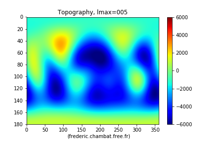
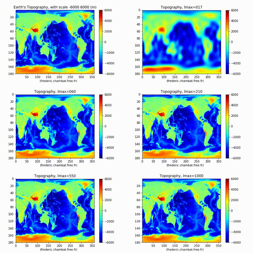
The image above illustrates the description of the Earth’s surface at order 5. The representation gives a very vague idea of the seas and continents.
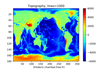
When sampled at order 1000, the description becomes precise enough to finely describe the Earth’s topography.
An analogy can be drawn — with due proportionality — by equating relief with acoustic pressure. More precisely, this would be the distribution of acoustic pressure on a sphere around the listener. Note that the local pressure variation at every point on this sphere is far more volatile over time.
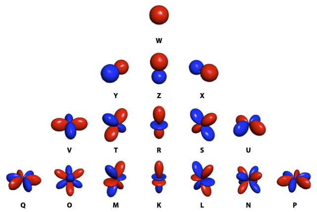
The image above shows only the harmonics up to order 3. We can see the complexity of their morphology. However, their combination allows 3D space to be observed in all directions with greater precision than at order 1, and thus allows that space to be encoded.
Ultimately, the challenge is to perform the inverse operation — decoding — in order to render the field, just as with topography. A major difference in the sonic domain: we cannot deploy as many loudspeakers as pixels!