
The “sound source localization” section describes the spectral localization cue related to the filtering performed by the shape of the head. This filtering is specific to each individual, each of their ears, and varies as a function of the angle of incidence of the acoustic wave. The brain integrates this difference to evaluate the angle of incidence.
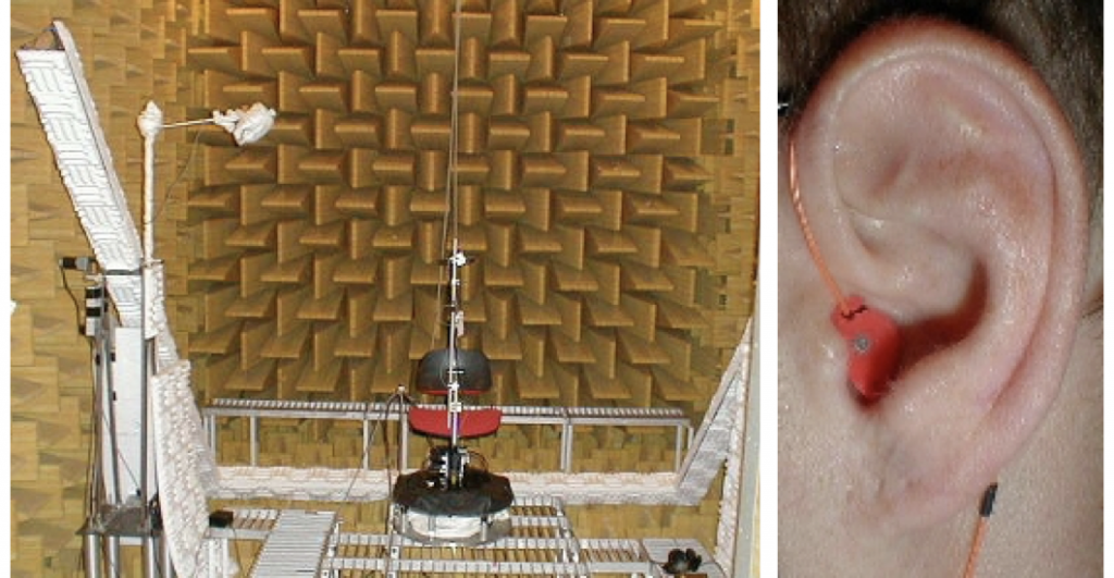
This filtering (referred to as a transfer function) can be measured in the form of impulse responses, IR[1], for different source positions around the listener. This set of measurements is described by the HRTF[2] (photos below). More precisely, these measurements collect the IRs related to the shape of the head. We then speak of HRIR (Head Related Impulse Response). While there is currently no truly practical solution for each person to measure their own HRTFs personally, several accessible measurement databases exist: Listen [3], ITA [4], Bili, Cipic, and more.
Binaural spatialization uses these HRTFs, or more precisely, the set of HRIRs measured, to create the illusion of 3D spatial audio over headphones: by applying these different filters (different for the left and right ears) as a function of the position of a virtual source.
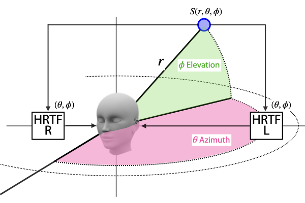
It is therefore important to understand that HRTFs are approximated by a set of measured HRIRs, which will be used by the algorithm as a function of a source’s position (azimuth and elevation). The use of HRIRs requires an operation with the source signal called a convolution product[6].
Binaural monitoring and binaural spatialization.
HOLOPHONIX provides by default a binaural reproduction of the spatialization performed on a loudspeaker array: accessible in the “monitoring” section. The algorithm takes each loudspeaker as a source. The user can simulate the spatialization performed on a diffusion system. This simulation does not replace the reality of spatialization on the diffusion system.
HOLOPHONIX allows binaural spatialization over headphones instead of a multi-loudspeaker diffusion system. Works intended for headphone listening can thus be produced. Unlike the monitoring system, each source is processed by the algorithm.
[1] Impulse Response: Sending an impulse signal to the input of a linear time-invariant system makes it possible to extract at its output the frequency profiles in amplitude and time (phase) that characterize this system. To simplify, this corresponds to a temporal fingerprint of a system.
[2]Head Related Transfer Function.
[3] A. Ircam, “Listen HRTF Database,” 2002-2003.: http://recherche.ircam.fr/equipes/salles/listen/download.html.
[4] R. Bomhardt, M. de la Fuente Klein and J. Fels, “The ITA HRTF-database – Institute for Hearing Technology and Acoustics,” 2016.: https://www.akustik.rwth-aachen.de/cms/Institut-fuer-Hoertechnik-und-Akustik/Forschung/~lsly/HRTF-Datenbank/?lidx=1.
[5] O. Warusfel, “Listen HRTF Database,” 2002.: http://recherche.ircam.fr/equipes/salles/listen/index.html.
[6] Not to be confused with the product of two quantities, this is a bilinear mathematical operator representing linear filtering. The convolution product (s*I) of a signal (s) and the impulse response (I) of a system gives the result of that signal passing through that system. It is often used in production for reverberation using an acoustic impulse response.